Custom reference state for the dimensional anelastic MHD formulation in a convective spherical shell based on polytropes
Problem Setup
We define the reference state of the convective region based on a polytrope that has a form given by
\(\rho=\rho_0 z^n\),
\(P=P_0 z^{n+1}\),
and
\(T=T_0 z\),
where \(\rho\), \(P\), and \(T\) are the density, pressure, and temperature respectively, and where the polytropic variable \(z\) is an as-of-yet undetermined function of radius. We further assume that these quantities are related by the ideal gas law, with
\(P=R\rho T\),
where \(R\) is the gas constant. It is related to the specific heats at constant pressure (\(c_p\)) and contant volume (\(c_v\)) through the relation
\(R=c_p-c_v=c_p(1-\frac{1}{\gamma})\),
with
\(\gamma\equiv \frac{c_p}{c_v}\).
For a monotomic ideal gas, we have that
\(\gamma\equiv \frac{5}{3}\).
Finally, we require that the polytrope satisfies hydrostatic balance. Namely,
\(\rho\frac{GM}{r^2}=-\frac{\partial P}{\partial r}\),
where \(G\) is the gravitational constant, and \(M\) is the mass of the star.
Polytropic Solution
Substituting our relations for \(P\), \(\rho\), and \(T\) into the equation of hydrostatic balance, we arive at
\(\frac{\partial z}{\partial r}= - \frac{GM}{(n+1)RT_0 r^2} = - \frac{2GM}{5(n+1)c_pT_0 r^2}\) .
This motivates us to seek a form for \(z\) of
\(z = a +\frac{b}{r}\),
and immediately, we see that b must be given by
\(b = \frac{2GM}{5(n+1)c_pT_0}\).
Note that while \(T_0\) remains undetermined, we can now compute \(\partial T/\partial r\). In order to determine \(a\), we need one more constraint. In our case, we will specify the number of density scaleheights, \(N_\rho\), across the convection zone. We denote the top of the convection zone by a subscript \(t\) and the base of the convection zone by a subscript \(b\). We then have \(N_\rho = \frac{ \rho_b }{ \rho_t } = \frac{z_b^n}{z_t^n}\),
or equivalently, using \(C\) to denote the exponential factor, and \(\beta \equiv \frac{r_b}{r_t}\), we have
\(C\equiv e^{\frac{N_\rho}{n}} = \frac{a+b/r_b}{a+b/r_t}\).
Rearranging, we find our expression for \(a\)
\(a = \frac{fb}{r_b}\),
where
\(f \equiv \frac{\beta C-1}{1-C}\).
This yields our expression for \(z\) in terms of \(T_0\)
\(z = b (\frac{1}{r} +\frac{f}{r_b} )= \frac{2GM}{5(n+1)c_pT_0}\left(\frac{1}{r} +\frac{f}{r_b} \right)\).
Factors of \(T_0\) cancel out, when calculating the temperature, leaving us with a complete description of its functional form. We are free to choose any value of \(T_0\) as a result; we use \(T_b\), the temperature at the base of the convection zone. We have that
\(T_0 = T_b = \frac{2GM}{5(n+1)c_p}\left(\frac{1+f}{r_b}\right)\),
completing our description of z. Values for \(\rho_0\) and \(P_0\) can now similarly be computed by enforcing the value of \(\rho\) and \(P\) as a particular point. As with \(T\), we choose the base of the convection zone in the code that follows.
[1]:
#######################
import numpy
import matplotlib.pyplot as plt
from matplotlib.pyplot import plot, draw, show

import os, sys
sys.path.insert(0, os.path.abspath('../../'))

import post_processing.reference_tools as rt # You will need the refernce_tools.py to run this notebook
import post_processing.rayleigh_diagnostics as rdiag
Matplotlib is building the font cache; this may take a moment.
[2]:
# Grid Parameters
# Here, we use solar values as an example

nr    = 512         # Number of radial points
ri    = 5e10        # Inner boundary of radial domain
ro    = 6.586e10    # Outer boundary of radial domain
rcz   = 5e10        # base of the CZ

#apsect ratio
beta=ri/ro

#Polytrope Parameters
ncz   = 1.5         # polytropic index of convection zone
nrho  = 3.          # number of density scaleheights across convection zone (not full domain)
mass  = 1.98891e33  # Mass of the star
G     = 6.67e-8     # gravitational constant
rhoi  = 0.18053428  # density at the base of convection zone
cp    = 3.5e8        # specific heat at constant pressure
gamma = 5.0/3.0     # Ratio of specific heats for ideal gas

lsun = 3.846e33     # solar luminosity for scaling the volumetric heating
[3]:
radius = numpy.linspace(ri,ro,nr) #Radial domain of the CZ
[4]:
#Compute a  CZ polytrope (see reference_tools)

poly1 = rt.gen_poly(radius,ncz,nrho,mass,rhoi,G,cp,rcz)
gas_constant = cp*(1.0-1.0/gamma)  # R

temperature= poly1.temperature # temperature T
density = poly1.density  # density rho
pressure = poly1.pressure # pressure P, this won't matter -- set it equal to something
dsdr = poly1.entropy_gradient # dS/dr
entropy= poly1.entropy # entropy S, this won't matter -- set it equal to something
dpdr = poly1.pressure_gradient # dP/dr
gravity= mass*G/radius**2  # gravity g
[5]:
# Calculation of the first and second derivative of lnrho and the first derivative of lnT.
# If we do not calculate those here, then they are calculated within Rayleigh!

d_density_dr = numpy.gradient(density,radius, edge_order=2)
dlnrho = d_density_dr/density
d2lnrho = numpy.gradient(dlnrho,radius, edge_order=2)
dtdr = numpy.gradient(temperature,radius, edge_order =2)
dlnt = dtdr/temperature
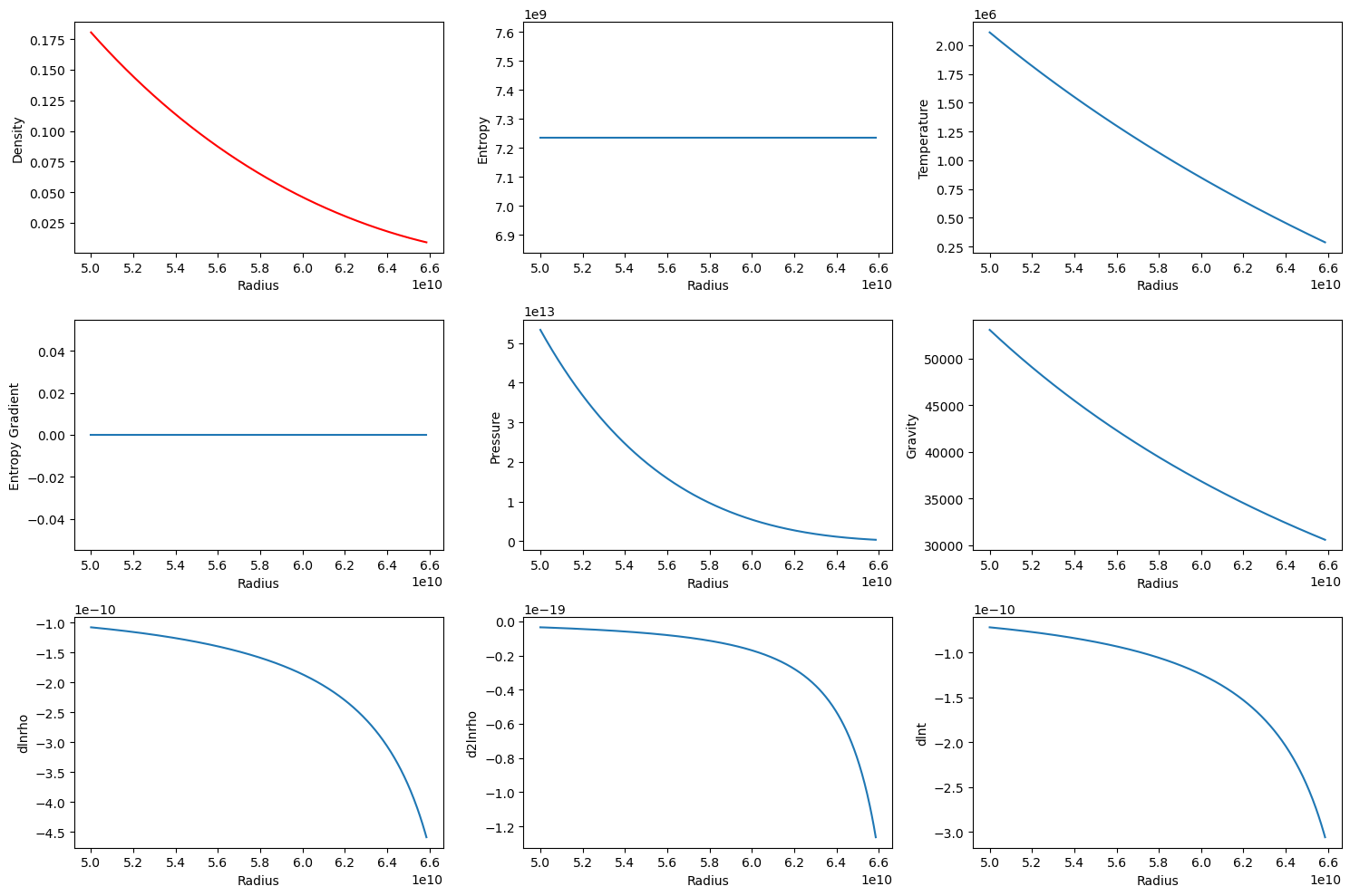
[6]:
# Plots of  the dimensional reference state profiles, i.e. the density profile, the temperature profile, etc.

fig, ax = plt.subplots(nrows =3,ncols = 3, figsize=(15,10) )
ax[0][0].plot(radius,density,'r')
ax[0][0].set_xlabel('Radius')
ax[0][0].set_ylabel('Density')

ax[0][1].plot(radius,entropy)
ax[0][1].set_xlabel('Radius')
ax[0][1].set_ylabel('Entropy')

ax[0][2].plot(radius,temperature)
ax[0][2].set_xlabel('Radius')
ax[0][2].set_ylabel('Temperature')

ax[1][0].plot(radius,dsdr)
ax[1][0].set_xlabel('Radius')
ax[1][0].set_ylabel('Entropy Gradient')

ax[1][1].plot(radius,pressure)
ax[1][1].set_xlabel('Radius')
ax[1][1].set_ylabel('Pressure')

ax[1][2].plot(radius,gravity)
ax[1][2].set_xlabel('Radius')
ax[1][2].set_ylabel('Gravity')

ax[2][0].plot(radius,dlnrho)
ax[2][0].set_xlabel('Radius')
ax[2][0].set_ylabel('dlnrho')

ax[2][1].plot(radius,d2lnrho)
ax[2][1].set_xlabel('Radius')
ax[2][1].set_ylabel('d2lnrho')

ax[2][2].plot(radius,dlnt)
ax[2][2].set_xlabel('Radius')
ax[2][2].set_ylabel('dlnt')

plt.tight_layout()

plt.show()
[7]:
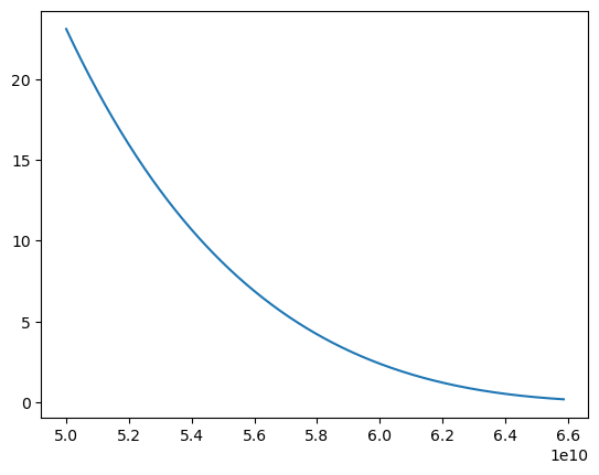
# Calculation of the heating profile based on the pressure, if we want to have a heating function in our setup.

hprofile = numpy.zeros(nr,dtype='float64')
hprofile[:] = pressure[:]

#################################################################
# We normalize the heating function so that it integrates to 1.

integrand= numpy.pi*4*radius*radius*hprofile
hint = numpy.trapz(integrand,x=radius)
hprofile = hprofile/hint
#plt.plot(radius,hprofile)
plt.plot(radius, hprofile*lsun)
[7]:
[<matplotlib.lines.Line2D at 0x7fab92ceb430>]
[8]:
my_ref = rt.equation_coefficients(radius)
[9]:
# Here we define all the functions and constants that will be written in our data file and
# read by Rayleigh if we choose the custom reference state (=4)

unity = numpy.ones(nr,dtype='float64')
buoy =density*gravity/cp # calculation of the buoyancy term used in the momentum equation

my_ref.set_function(density,1) # density rho
my_ref.set_function(buoy,2)    # buoyancy term
my_ref.set_function(unity,3)   # nu(r) -- can be overwritten via nu_type in Rayleigh
my_ref.set_function(temperature,4) # temperature T
my_ref.set_function(unity,5)  # kappa(r) -- works like nu
my_ref.set_function(hprofile,6)  # heating -- this is normalized to one

my_ref.set_function(dlnrho,8)  # dlnrho/dr
my_ref.set_function(d2lnrho,9) # d^2lnrho/dr^2
my_ref.set_function(dlnt,10)   # dlnT/dr
my_ref.set_function(unity,7)  # eta -- works like nu and kappa --  magnetic diffusivity
my_ref.set_function(dsdr,14)   # dS/dr

# The constants can all be set/overridden in the input file
# NOTE that they default to ZERO, but we want
# most of them to be UNITY.
# These aren't very useful in the dimensional anelastic formulation but are VERY useful
# for the non-dimensional version of the anelastic custom reference state!

my_ref.set_constant(1.0,1)  # multiplies the Coriolis force--Should be 2 Omega (complication here)
my_ref.set_constant(1.0,2)  # multiplies buoyancy
my_ref.set_constant(1.0,3)  # multiplies pressure gradient
my_ref.set_constant(0.0,4)  # multiplies lorentz force
my_ref.set_constant(1.0,5)  # multiplies viscosity
my_ref.set_constant(1.0,6)  # multiplies entropy diffusion (kappa)
my_ref.set_constant(0.0,7)  # multiplies eta in induction equation
my_ref.set_constant(1.0,8)  # multiplies viscous heating
my_ref.set_constant(1.0,9)  # multiplies ohmic heating
my_ref.set_constant(lsun,10) # multiplies the heating (if normalized to 1, this should be the luminosity)
my_ref.write('dimensional.dat')  # Here we write our data file to be used to run our simulation with Rayleigh!
print(my_ref.fset)
print(my_ref.cset)
[1 1 1 1 1 1 1 1 1 1 0 0 0 1]
[1 1 1 1 1 1 1 1 1 1]
[10]:
# Once you've run for one time step, set have_run = True !!

# Here we check if the output reference state is the same as the one we used as an input (sanity check)

# NOTE: We need the output file "equation_coefficients" to run this, as well as the PDE_Coefficients
# from rayleigh_diagnostics.py

try:
    cref = rdiag.PDE_Coefficients() # This will give us the output reference state
    have_run = True
except:
    have_run = False

if (have_run):

    fig, ax = plt.subplots(ncols=3,nrows=4, figsize=(16,4*4))
    # density, derivatives of lnrho
    ax[0][0].plot(cref.radius,cref.density,'yo')
    ax[0][0].plot(radius,density)
    ax[0][0].set_xlabel('Radius (cm)')
    ax[0][0].set_title('Density')

    ax[0][1].plot(cref.radius, cref.dlnrho,'yo')
    ax[0][1].plot(radius, dlnrho)
    ax[0][1].set_xlabel('Radius (cm)')
    ax[0][1].set_title('Log density gradient')

    ax[0][2].plot(cref.radius,cref.d2lnrho,'yo')
    ax[0][2].plot(radius,d2lnrho)
    ax[0][2].set_xlabel('Radius (cm)')
    ax[0][2].set_title('d_dr{Log density gradient}')

    # temperature and derivative of lnT
    ax[1][0].plot(cref.radius,cref.temperature,'yo')
    ax[1][0].plot(radius,temperature)
    ax[1][0].set_xlabel('Radius (cm)')
    ax[1][0].set_title('Temperature')

    ax[1][1].plot(cref.radius, cref.dlnT,'yo')
    ax[1][1].plot(radius, dlnt)
    ax[1][1].set_xlabel('Radius (cm)')
    ax[1][1].set_title('Log temperature gradient')

    # entropy gradient
    ax[2][1].plot(cref.radius, cref.dsdr,'yo')
    ax[2][1].plot(radius, dsdr,'b')
    ax[2][1].set_xlabel('Radius (cm)')
    ax[2][1].set_title('Entropy gradient')

    # Note that you must build the buoyancy term from the functions/constants
    ax[3][1].plot(cref.radius, cref.functions[:,1]*cref.constants[1],'yo')
    ax[3][1].plot(radius, gravity*density/cp)
    ax[3][1].set_xlabel('Radius (cm)')
    ax[3][1].set_title('Buoyancy')

    # Note that the output heating (cref.heating) is hprofile/density/temperature*luminosity
    ax[3][2].plot(cref.radius, cref.heating*cref.rho*cref.T,'yo')
    ax[3][2].plot(radius, hprofile*lsun)
    ax[3][2].set_xlabel('Radius (cm)')
    ax[3][2].set_title('Heating')

    plt.tight_layout()
    plt.show()
[ ]: